Customizing Size and Background on 2-D Plots

Two new options, background and size for 2-D plotting commands, allow you to superimpose a plot on a background image, set a background color or specify the size of the plot window.

>

Setting the Size of the Plot Window

Example

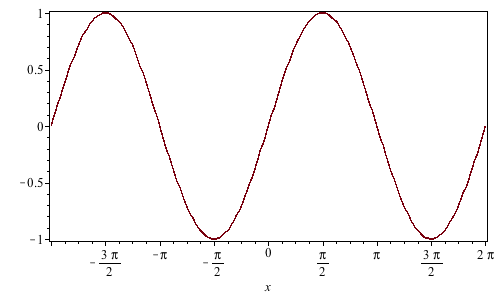
The width and height of the plot window can be given as the number of pixels. >

Example

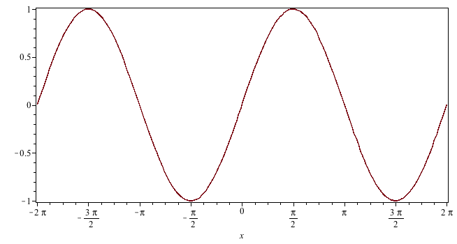
If the width is given as a floating-point number, it is interpreted as a proportion of the worksheet width.  >

Example

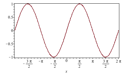
If the height is given as a floating-point number, it is interpreted as the ratio of the height to the width. The height can be the special name "golden"; in this case, the height/width ratio is the reciprocal of the golden ratio.  >

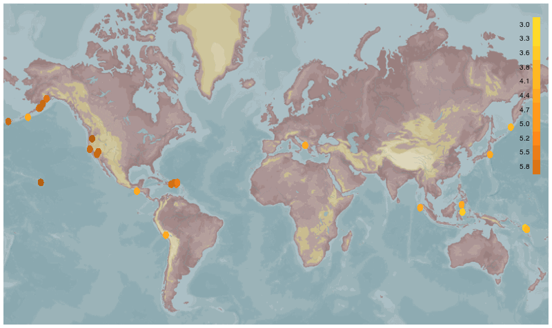
Using an Image as the Background

The image can be specified as either a name (string) of an image file or an image (array) usable by the package. By default, the plot is displayed with the dimensions of the image.

Example

The following example shows the location of all earthquakes of magnitude 2.5 or greater over a seven day period.  Reference: Data compiled by the U.S. Geological Survey. >

 

Example

An image that can be produced or used with the ImageTools package can also be used as the background. The Fractals package can also produce such images. >   >   >   >     >     >     >

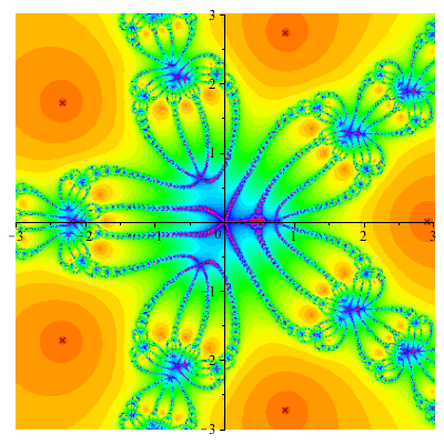
Setting a Background Color

The background option can also be used to set the background color.

Example

>

>