Custom Plot Shading

A number of improvements have been made to the custom coloring of plot surfaces. These include new options for the plot3d command and substantial updates to the surfdata command.

Shading can be specified using coloring procedures, color data from existing 3-D plots, or images.

Shading Schemes for Surfaces

The Colorscheme Option

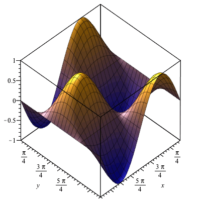
A new colorscheme option allows custom shading of 3-D plots when using the plot3d command.
In this example, the shading is according to the height with a color gradient from medium blue through orange. 

>	plot3d(sin(x)*cos(y), x=0..2*Pi, y=0..2*Pi, colorscheme=["MediumBlue", "Orange"]);

   

In the next example, we will display the default shading scheme alongside a custom z-gradient shading scheme that specifies the colors in use, the breakpoints at which shades are switched, and the colorspace through which the color gradients are taken. 

>	p1 := plot3d(sin(x)*cos(y), x=0..2*Pi, y=0..2*Pi): p2 := plot3d(sin(x)*cos(y), x=0..2*Pi, y=0..2*Pi, colorscheme=["zgradient",    ["DarkBlue", "LightBlue", "Purple", "Yellow"], markers=[0, .3, .6, 1],    colorspace="RGB"] ): plots:-display(Array([p1, p2]));

   

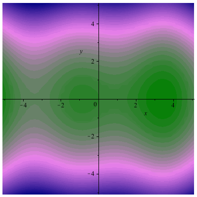
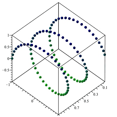
The new colorscheme option can also be used with plots created by the plots:-densityplot, plots:-pointplot, and plots:-pointplot3d commands. 

>	plots:-densityplot(x*cos(x)+y^2, x=-5..5, y=-5..5, colorscheme=["Green", "Violet", "NavyBlue"], style=surface);

   

>	plots:-pointplot3d([seq([i/100, cos(i*Pi/20), sin(i*Pi/20)], i=1..100)], symbol=solidcircle, symbolsize=20, colorscheme=["LimeGreen", "NavyBlue"]);

   

The Image Option

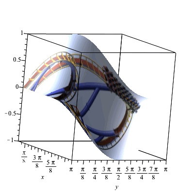
Images can be used for the shading of a surface with the image=t option. The value t may be an image data Array or the name of an image file. This option is available with the plot3d command, the plots:-surfdata command (as described below) and with other 3-D plotting commands that use plot3d to generate their results.

>	with(ImageTools): imgdir := cat(kernelopts(mapledir), "/data/images/"):

 

>	imgfile := cat(imgdir, "rollercoaster.jpg"):

>	plot3d(sin(y)*cos(x), x=0..Pi, y=0..Pi, image=imgfile, lightmodel=none, orientation=[0, 80, 30]);

 

Reusing Color Data From 3-D Plots

The following example requires an understanding of plot data structures, as described in the plot/structure help page. The COLOR substructure generated by a call to the plot3d command can be reused for shading in a subsequent call.

>	P := plot3d(x*exp(-x^2-y^2), x=-2..2, y=-2.. 2, color=[.6, abs((1/4)*x), abs((1/2)*y)]): P;

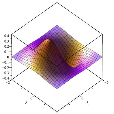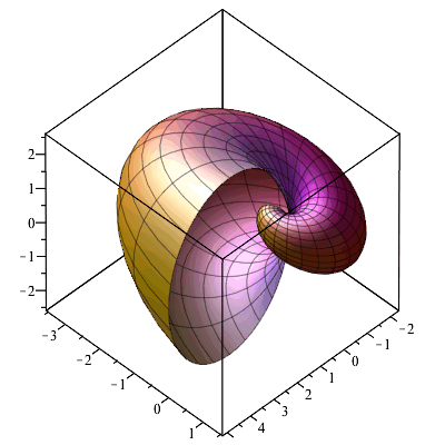
Extract the COLOR substructure, and reuse it in a new call to the plot3d command. 

Note that the first pair of dimensions of the reused data Array has to be at least as large as the grid size in the subsequent call. In the next example, both plot3d calls use the default value of grid=[49,49]. 

>	A := op([1, 4], P);

>	plot3d(1.3^x*sin(y), x=-1..2*Pi, y=0..Pi, coords=spherical, color=A);

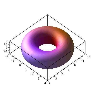
In the next example, the torus is created with the grid=[49,49] option, so as to match the reused color data Array. 

>	plots:-display(plottools:-torus([1, 1, 1], 1, 2, grid=[49, 49], color=A),     scaling=constrained, style=surface);

Improvements to Plots:-surfdata

Option to Produce 2-D Plots

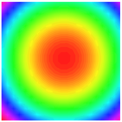
The surfdata command now accepts the option dimension=2 as a way to specify that the result will be a 2-D plot. This allows a coloring scheme to be rendered on a flat, rectangular display, analogous to a 2-D density plot.

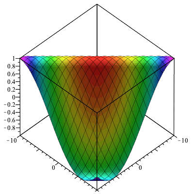
First let's generate the usual 3-D surface produced by the surfdata command, using a coloring procedure. 

>	cosdata := [seq([seq([i, j, evalf(cos((i+j)*(1/5)))], i=-10..10)], j=-10..10)]: plots:-surfdata( cosdata, color = proc(x, y) x^2+y^2 end proc);

Now we'll generate a 2-D plot, using the same coloring procedure. 

>	plots:-surfdata(cosdata, color=proc(x, y) x^2+y^2 end proc, dimension=2, axes=none, style=surface);

The Colorscheme Option

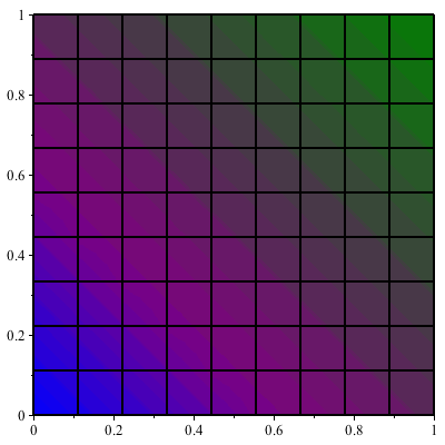
The surfdata command has been updated to accept the new colorscheme option, as described above.

>	plots:-surfdata(Matrix(10, 10, (i,j) -> i+j), dimension=2,    colorscheme=["zgradient", ["Blue", "Purple", "Green"], markers=[0, .3, 1]]);

Shading with an Image

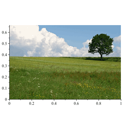
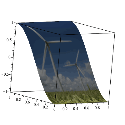
An image can be used to color the surface. In addition, certain options (dimensions, scaling, and style) are set automatically with the image option. These options can be overridden.

 

Note that the first argument of surfdata is now optional in cases where an image is provided. In this situation, the plot's default is assumed to be 2-D.

>	imgfile := cat(kernelopts(mapledir),"/data/images/", "tree.jpg"): plots:-surfdata(image=imgfile);

>	imgarr := Scale( Read( cat(imgdir, "windturbine.jpg" ) ),1/3 );

>	plots:-surfdata(Matrix(Width(imgarr), Height(imgarr),    (i,j)->evalf(cos((1-(1/Height(imgarr))*j)*Pi)), datatype=float[8]),    image=imgarr, lightmodel=none, orientation=[-100, 80, 30], axes=box);

View a Recorded Webinar • Custom Plot Shading in Maple